R: Cluster Analysis

# lib(s): pvclust, mclust

# Red indicates stuff ya gotta to edit.

# Essentially reposted from: http://www.statmethods.net/advstats/cluster.html

# Data input: generic

# infile (as mentioned in the script below) should contain all the variables you want to analyze, and nothin else.

# remove/estimate missing data and/or rescale variables for compatibilty
infile <- na.omit(infile) # listwise deletion of missing
infile <- scale(infile) # standardize variables

# - K-MEANS - alpha tested ok on 23Sept2010

# Determine number of clusters
wss <- (nrow(infile)-1)*sum(apply(infile,2,var))
for (i in 2:15) wss[i] <- sum(kmeans(infile,
centers=i)$withinss)
plot(1:15, wss, type="b", xlab="Number of Clusters",
ylab="Within groups sum of squares")

# K-Means Cluster Analysis
fit <- kmeans(infile, 5) # 5 cluster solution
# get cluster means
aggregate(infile,by=list(fit$cluster),FUN=mean)
# append cluster assignment
infile <- data.frame(infile, fit$cluster)

# - END OF K-MEANS -

# - Hierarchical Agglomerative - alpha tested ok on 23Sept2010

# Ward Hierarchical Clustering
d <- dist(infile, method = "euclidean") # distance matrix
fit <- hclust(d, method="ward")
plot(fit) # display dendogram
groups <- cutree(fit, k=5) # cut tree into 5 clusters
# draw dendrogram with red borders around the 5 clusters
rect.hclust(fit, k=5, border="red") 

#  - Hierarchical Agglomerative - FULL DEMO

# If you can't do data handling on R, do it on excel or something. 
# Your data gotta look like this (I ran the demo on this data):

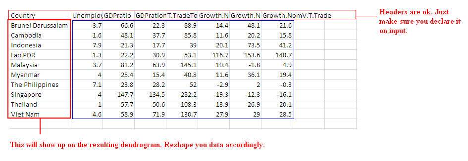
# If your data's set up right, here's the minimal script you need:
infile <- read.csv("E:/AseanDat.csv",header=T)
library(pls)
neo <- as.matrix(infile[,-1])
neo.std <- stdize(neo)
neo.dist <- dist(neo.std, method = "euclidean") # distance matrix
fit <- hclust(neo.dist, method="complete")
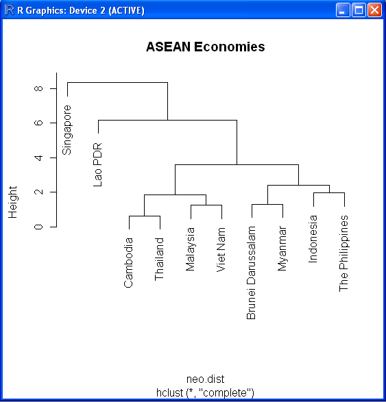
plot(fit,labels=infile$Country,main="ASEAN Economies") # display dendrogram


The dendrogram will look like this:

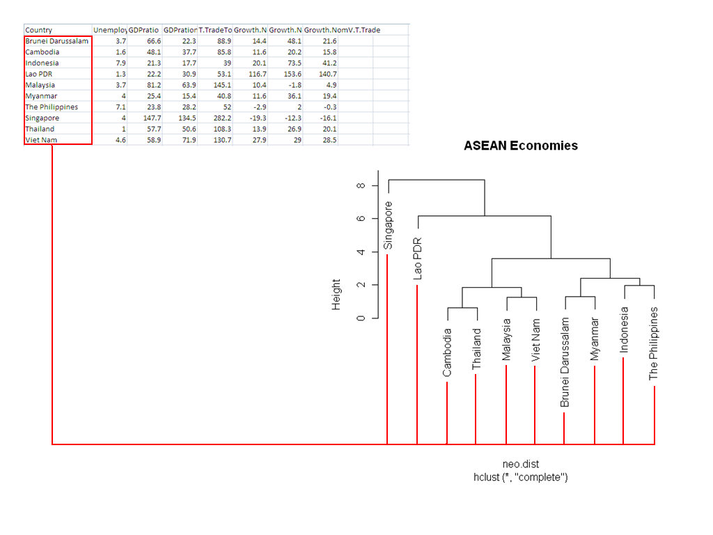
Note how it relates back to the input data:

# You can draw boxes around the clusters with R - if you want R to show x number of groups:

# draw dendogram with red borders around the major clusters

rect.hclust(fit, k=4, border="red")  # in this case, the 4 main groups are highlighted.

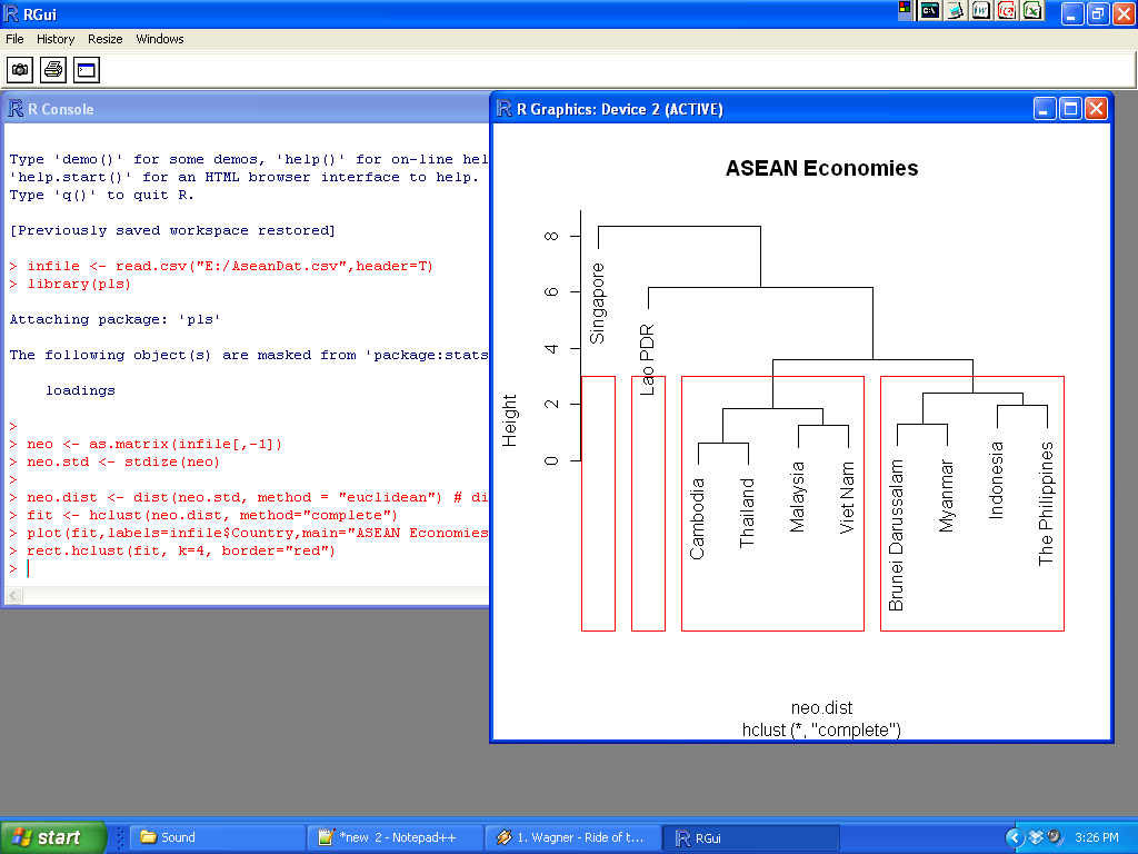
# ... sometimes, R doesn't do a very good job - if that's the case(like in this example), just copy the output and put the boxes in yourself using whatever graphics editing software you want.

# Ward Hierarchical Clustering with Bootstrapped p values

library(pvclust)
fit <- pvclust(infile, method.hclust="ward",
method.dist="euclidean")
plot(fit) # dendogram with p values
# add rectangles around groups highly supported by the data
pvrect(fit, alpha=.95)

# - END OF HIERARCHICAL AGGLOMERATIVE -

# - MODEL-BASED - alpha tested ok on 23Sept2010
# Model Based Clustering

library(mclust)
fit <- Mclust(infile)
plot(fit, infile) # plot results
print(fit) # display the best model

# - END OF MODEL-BASED -

# - Possible Means of Visualising of Results - alpha tested ok on 23Sept2010

# K-Means Clustering with 5 clusters
fit <- kmeans(infile, 5)

# Cluster Plot against 1st 2 principal components
# vary parameters for most readable graph
library(cluster)
clusplot(infile, fit$cluster, color=TRUE, shade=TRUE,
labels=2, lines=0)

# Centroid Plot against 1st 2 discriminant functions
library(fpc)
plotcluster(infile, fit$cluster)

# - END OF RESULT VISUALISATION -

# - SOLUTION VALIDATION -

# comparing 2 cluster solutions - alpha tested ok on 23Sept2010
library(fpc)
cluster.stats(d, fit1$cluster, fit2$cluster)

# - END OF SOLUTION VALIDATION -

# /* END OF CLUSTER ANALYSIS */